The BS 7910 Fracture Component | Deep Dive

In This Article
The BS 7910 Fracture Component automates the methods described in BS 7910:2019 for unstable fracture. This article provides a detailed description about the Component, its options, and settings. The user is expected to be familiar with BS 7910 and should reference their own copy of the document, as appropriate. The topics are covered in this article include the following:
- Overview
- Implementation of the BS 7910 Solutions
- Failure Assessment Diagrams (FADs)
- Creating a New Fracture Component
- Geometry Input and Options
- Load Input and Options
- Tensile Input and Options
- Toughness Input and Options
- Component Settings and Options
- Running a Fracture Component and Viewing the Results
- The Fracture Report
- Exporting Results as MS Excel Files
- Running an Embedded Flaw
- Running the Solver and Viewing the Results
- Running a Batch of Flaws and Viewing the Results
- Creating a Second Fracture Component by Duplicating and Editing the First
Overview
The BS 7910 Fracture Component assesses the acceptability of a crack-like flaw consistent with the methods described BS 7910:2019 Clause 7, Annex M, and Annex P. In general, for each assessment, three values are calculated: the fracture ratio (Kr), load ratio (Lr), and the failure assessment line (FAL). On the Failure Assessment Diagram (FAD), if the assessment point based on the Kr and Lr values, is beneath the FAL, the flaw is assessed as acceptable. If the assessment point is on the FAL, the flaw is assessed as critical, or if the assessment point is above the FAL, the flaw is assessed as not acceptable. The following illustration from Material ECA is an example of a Failure Assessment Diagram (FAD) for an acceptable flaw showing the assessment point is below the Failure Assessment Line.

Implementation of the BS 7910 Solutions
BS 7910:2019 provides several methods for calculating the Fracture Ratio (Kr) and Load Ratio (Lr) depending on the Geometry Type selected. The Geometry Type property is more thoroughly described in the article for Material ECA Components. The following table lists the Geometry Types available, and the BS 7910 solutions used by Material ECA.
| Geometry Type | Flaw Type | Fracture Ratio Solution | Load Ratio Solution |
| Plate | Surface | M.4.1 | P.5.1 |
| Embedded | M.4.5 | P.5.3 | |
| Plate Corner | Surface | M.5.1 | P.6.1 |
| Circumferential OD | Surface | M.6 or M.7.3.4 | P.9.4 |
| Embedded | M.4.5 | P.5.3 | |
| Circumferential ID | Surface | M.6 or M.7.3.2 | P.9.2 |
| Embedded | M.4.5 | P.5.3 | |
| Axial OD | Surface | M.6 or M.7.2.4 | P.8.4 |
| Embedded | M.4.5 | P.5.3 | |
| Axial ID | Surface | M.6 or M.7.2.2 | P.8.2 |
| Embedded | M.4.5 | P.5.3 | |
| Round Straight | Surface Straight | M.10.1 | P.12.1 |
Because the fracture ratio (Kr) value varies along the crack front, each time a Fracture component is run multiple Kr values are calculated. From these, the largest Kr value is selected to determine the acceptability of the flaw, and the associated flaw angle is reported in the results. By default, the number of Kr values calculated is 46, which is every 2 degrees from the surface to the deepest locations (0 to 90 degrees). The M.7 solutions are an exception; Annex M.7 only provides for calculations at the surface and deepest points (2 points).
Material ECA Fracture Component allows the user to input different values of toughness for surface and embedded flaws. Furthermore, for surface flaws, the user can input multiple values of toughness based on distance to the surface. For example, for assessing carbon steel pipe internally clad with alloy 625, the toughness associated with the first 3 mm (cladding thickness) can have one toughness value, the remaining thickness (associated with carbon steel) can have another value. There is no limit to the number of layers and toughness values; however, if the M.7 solution is used, only the surface and deepest points on the flaw will be assessed.
Failure Assessment Options
Material ECA provides three options: Option 1 Continuous, Option 1 Discontinuous, and Option 2, as described in BS 7910:2019; Claus 7. For Option 2, the user will be required to input the appropriate engineering stress-strain curve. For Option 1 Discontinuous, the user will be required to input the strain associated with the Luder’s Plateau.
Creating a New Fracture Component
Navigate to the Components page in the desired Project, then click on the tile with the plus sign.

This will present the Add New Component form. Under Component Type, select Fracture. Under Method Type, Select BS7910:2019 Fracture. Under Name, input the desired name for the Component. Under Description, add a meaningful description of the Component.

Finally, click the Save button, and you will be returned to the Components page.
Open the new Component by clicking on it. This will allow you to input desired data, as described in the following sections.
Geometry Input and Options

Depending on the Geometry Type selected, the required input will vary. The above illustration shows the input required for a circumferential flaw on or near the ID surface of a pipe or cylinder – the Geometry Type is set to Circumferential ID. The required input will be Wall Thickness (B) and Outside Diameter (OD). Because the option to Automatically Calculate the Section Width (W) is selected, Material ECA will calculate the circumference based on the inside diameter and use that as the Section Width (W). If the option is not selected, an input will be available for the user to input the Section Width. The user may choose the units for each (mm or inches). Here the user chooses inches for Outside Diameter, and mm for wall thickness.
The user may input values for Km, Ktm, Ktb, and L. Each of these are implemented as described in BS 7910, Annex K. Km is usually used to address additional bending stress due to misalignment at a weld. Material ECA calculates the additional bending stress and uses it in both the fracture ratio (Kr) and load ratio (Lr) calculations.
Loading Input and Options
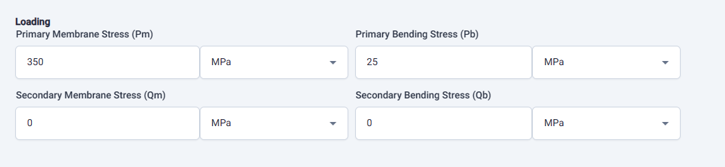
BS 7910 describes how to input primary and secondary membrane and bending stresses. The user may choose between ksi and MPa units for each item. Later, in the Settings section the user can choose to Relax Weld Residual Stresses. If so, the value input for Yield strength will be used by Material ECA to calculate the Secondary Membrane Stress (Qm), in which case the user may leave the values for Qm and Qb set to default, as they are not needed.
Tensile Material Input and Options
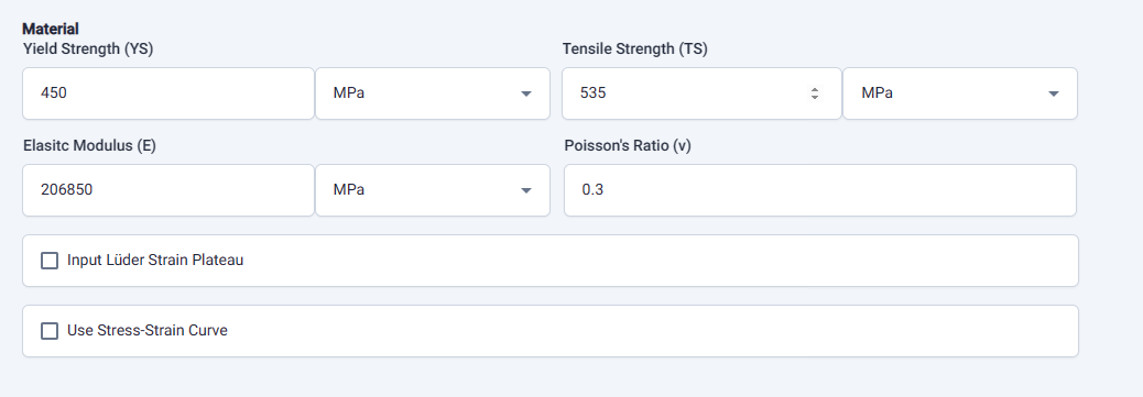
Values for the tensile material properties Yield and Tensile Strength, elastic modulus, and Poisson’s ratio are input here. Like stress, the user can choose between ksi or MPa units. These are the only input needed for a Type 1 Continuous Failure Assessment Diagram.
Selecting “Input Luder Strain Plateau” will allow the user to input the strain value associated with the Luder’s Plateau, which is needed for the Type 1 Discontinuous Failure Assessment Diagram. The user can choose between DL/L or % units.

Option 2 failure assessment diagrams (FAD) need a stress-strain curve. To enter data for a stress-strain curve, select “Use Stress-Strain Curve” and then “Paste Engineering Stress-Strain Curve”. That exposes a text box area for the stress-strain curve points as illustrated here.

Most use an Excel spreadsheet to process stress-strain curve data points and copy and paste them directly from the spreadsheet.
The values must be pasted such that each row is a pair – stress followed by strain values. The two values can be separated by a space, tab, comma, or any combination. This illustration shows stress is separated from strain by a tab as it appears when pasted directly from Excel. The units chosen are MPa and %.
There are three criteria all of which must be satisfied for a valid stress-strain curve:
- The first row must be 0, 0 (setting the origin)
- Strain values must incrementally increase
- Stress values must not incrementally decrease
Selecting the View Curve check box will display a chart of the input stress-strain curve, which allows the user to confirm the input before running the Component. Clicking the Validate Curve button will present a message saying whether the input is valid or including an error message.
Toughness Input and Options
Toughness may be input as either of three types:
- Stress Intensity (K) with units of ksi-in1/2, MPa-m1/2, or MPa-mm1/2
- J-Integral with units of kJ/m2, ksi-in, or in-lb/in
- CTOD with units of mm or inch
Users may input different values for toughness for surface and embedded flaws. The following figure shows how to set the toughness for both surface and embedded flaws to the same CTOD value of 0.25mm.
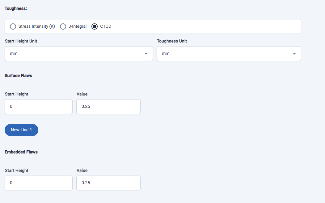
For surface flaws, users may input different values of toughness depending on the distance from the surface. The following screenshot shows how to set the toughness for surface flaws within 3mm of the surface to a CTOD value of 1.25mm and beyond that to a CTOD value of 0.25mm, which may be representative of a carbon steel pipe internally clad with Alloy 625, for example. The New Line button provides the input for additional layers of toughness.

On the first line, the value for Start Height must be set to 0.
Fracture Settings and Options
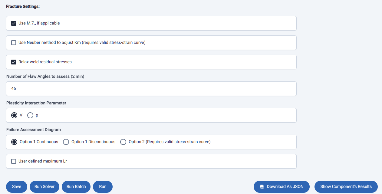
When Geometry Type is set to Circumferential or Axial flaws in cylinders or pipe, the Use M.7 option is enabled. The M.7 solutions are limited to a narrower range of wall thickness to diameter (t/D) ratios and flaw sizes. When selected, Material ECA will check if the M.7 solutions is allowed, and will use it if it is. Otherwise, it will use the M.6 solution.
DNV RP-F108 describes the Nueber method for adjusting the Km values due to plasticity at load levels approaching or exceeding the yield strength. Choosing this option requires the user to input a stress-strain curve. The results include the modified Km value used for the calculation.
Relaxing Weld Residual Stresses is described in BS 7910:2019; Clause 7.1.10.2. Selecting this option replaces the Secondary Membrane (Qm) and Bending (Qb) values inputs and automatically calculates a Qm value, as appropriate. The results include the modified Qm and Qb values used for the calculation.
The default number of Kr values calculated is 46, which is every 2 degrees from the surface to deepest points on the flaw (0 to 90 degrees), should be sufficient for most applications. The user may increase or decrease that value as desired is a range of 2 to 1000. For example, when assessing multiple material toughness layers and values, as described earlier, the user may choose to increase the Number of Flaw Angles, as appropriate. However, the M.7 solutions will only calculate values for the surface and deepest points, only 2 flaw angles will be assessed regardless of the input value.
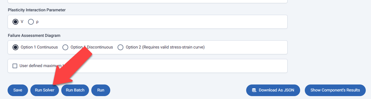
BS 7910:2019 provides two methods for addressing plasticity interaction between primary and secondary stresses, as described in Clause 7.3.6. The user may choose either method: V or r.
The user may choose one of three failure assessment diagram types: Option 1 Continuous, Option 1 Discontinuous, and Option 2. Option 1 Discontinuous will require the user to input the strain value associated with the Luders plateau, and Option 2 will require the user to input a stress-strain curve.
Finally, the user may input a custom value for maximum Lr.
When input is complete, click the Save button.
Clicking the Run button will assess a single flaw.
Clicking the Run Batch button will assess multiple flaws.
Clicking the Run Solver button will automatically calculate the critical flaws, which are those flaws that lie on the line separating acceptable flaws from not acceptable flaws on a Flaw Height vs Flaw Length chart.
Clicking the Download As JSON button, produces a file and save it in your local Download directory, depending on your local settings, representing the input data for the Component in JSON format. JSON formatted data is readily understood by most modern programming languages to facilitate custom pre or post processing.
When the Component is run and results are produced, they viewed from the Results directory. Clicking the Show Component Results button is one way the user can see the results.
Running a Fracture Component and Viewing the Results
In this section we’ll run the Fracture Component we just created and run it using a surface flaw with a height (a) of 3mm and a length (2c) of 12mm.
Click the Run button.

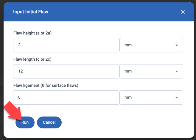
The Input Initial Flaw form appears. Enter 3mm for the Flaw Height, 12mm for the Flaw Length, and 0 for the Flaw Ligament. The Flaw Ligament is used to describe the minimum distance embedded flaws are from the surface. Setting Flaw Ligament to 0 lets Material ECA know a surface flaw is being assessed. Click the Run button.
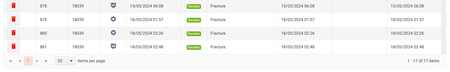
Navigate to the Results page for the Fracture Component created as shown in the following illustration.

Let’s explore the Results page. The Project containing this Component is Live Demonstration. Selecting Results from the menu on the left displays a list of results organized by the Component. The Component run was Fracture 01. The most recent Result is the one we want to view, but before we do let’s discuss the Status column.
We see the status was Success and colored green, which means it has run and returned results. If the status is Calculating and colored blue, the run was submitted to the Material ECA workstation, and the results have not yet been received. Even the most complicated Fracture components are processed by the workstation in less than a second, but it may take a few seconds to return the data via the internet depending on other factors. Try refreshing the browser and within a few seconds the status should change to Success.
If the status is Pending, that means the job has been placed in the queue, but the workstation has not yet picked it up. This could mean that the workstation is busy with other jobs, or the workstation is down for maintenance. Again, try refreshing the browser. If the status does not change within a few minutes, please let us know. Our contact information is available in the footer below and on the MaterialEnergies.com website.
The results can be deleted by clicking the red trash can icon in the Action column on the left.
Click anywhere else on the most recent result row to view the results page. Scrolling down is needed to display the entire page.

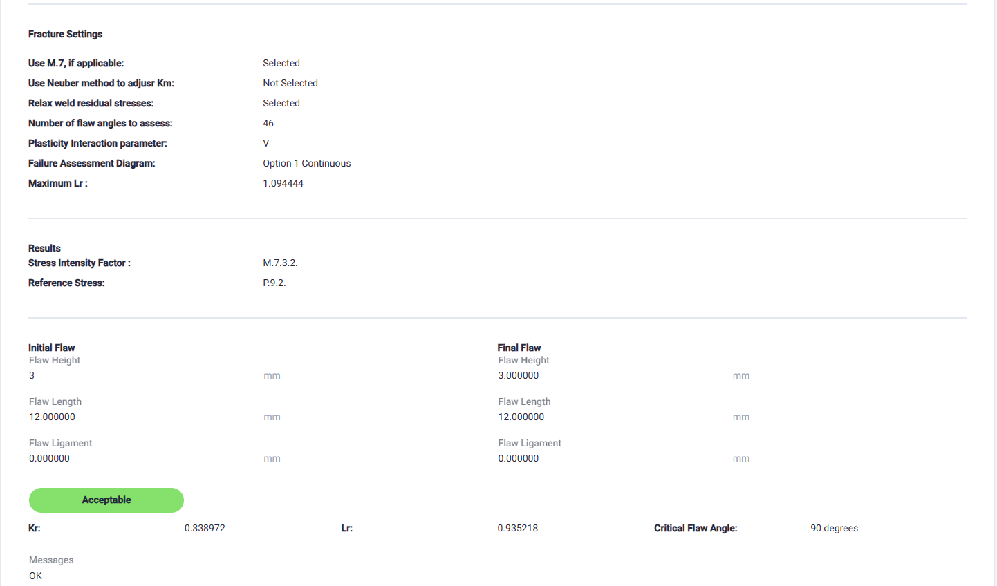
The top of the results page provides an overview, including the acceptability of the initial flaw, fracture ratio (Kr), load ratio (Lr), critical flaw angle, and the solutions used. In this case the solutions used were M.7.3.2 and P.9.2 from BS 7910, and the deepest point of the flaw (90 degrees) was associated with the largest fracture ratio (Kr).
Next the initial and final flaws are presented. Because unstable fracture does not calculate any flaw growth, the final flaw is the same as the initial flaw. Other components, such as fatigue crack growth, ductile tearing, and chain and group components that contain fatigue and tearing components will have larger final flaws than initial flaws.
Scrolling down displays the failure assessment diagram (FAD), where the assessment point, which is the calculated Kr and Lr values, are plotted with the failure assessment line. In this case, the assessment point is below the failure assessment line, so the assessment is acceptable. The chart is interactive. When you hover your mouse over the assessment point or the failure assessment line, the associated Kr and Lr values are displayed.

Scrolling farther down displays the calculation details. The Section Width (W) used was calculated in this case is associated with the circumference of the inside diameter. The Km used was input in this case; however, if the Nueber method was selected, the value used would be calculated. The Secondary stresses (Qm and Qb) used were calculated, as described earlier since the option to Relax Weld Residual Stresses was selected.
As mentioned earlier, the fracture ratio (Kr) was calculated at 46 locations along the flaw from surface (0 degrees) to the deepest point (90 degrees). The Stress Intensity Factor Details table lists the intermediate calculated values for for each flaw angle. In this case only the surface and deepest points have Kr values other than zero, because all M.7. solutions only provide stress intensity solutions for the surface and deepest points.
The table has the following columns, each are defined in BS 7910 Annex M:
- Flaw Angle (radians)
- Fracture Ratio (Kr)
- KI Primary (K1P, stress intensity factor associated with the primary stresses)
- KI Secondary (K1S; stress intensity factor associated with secondary stresses)
- Rho (r) and V: secondary stress interaction factors only one used as selected by the user
- Kmat: toughness value used (MPa mm1/2; when the user inputs multiple toughness values based on depth from the surface, different Kmat values will be presented based on the depth at the point on the flaw, as appropriate)
- Mk Is 3D: if true the 3D Mk solution was used
- Z is the depth from the surface in mm
- The other parameters are all defined in BS 7910 Annex M

The buttons below function as follows:
View Report Displays a summary of the input and results in a format suitable for printing and documentation. The report can be saved as a PDF file and will be discussed in the next section.
View Component returns the view to the Component input form.
Export As JSON formats the detailed results and input data into JSON format and exports the file to the local Downloads folder, depending on the settings of the local computer. Exporting results as JSON allows the most flexible and powerful way to post-process and use data generated by Material ECA. This is discussed more fully in another article.
Export As Excel formats the results and input data into an Excel file and exports the file to the local Downloads folder, depending on the settings of the local computer. This will be discussed later in this article.
The Fracture Report
From the Results view, clicking the View Report button displays the Report page. The Fracture Report serves as a method for documenting the calculation by presenting details about the calculation, all pertinent input data, and a summary of the results. The Fracture Report can be exported as a PDF file and saved, printed, and/or distributed.


Exporting Results to MS Excel
Returning to the Results page, clicking the Export As Excel button on the bottom of the page will process the detailed results into an Excel file and export it to your local Downloads folder, depending on the settings of your local computer. Exporting results as an Excel file serves as an alternate way to document results in a format suitable for some post-processing and charting.
The exported Excel file has two worksheets, one associated with the results, and another associated with the input. The following image shows the Fracture Results page.

The following image shows the Fracture Input page.

Running and Embedded Flaw
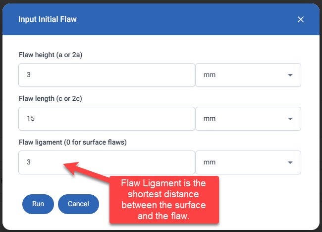
Return to the Component, scroll to the bottom of the page, and click the Run button. This time we’ll assess an embedded initial flaw. The Input Initial Flaw form appears, this time input a Flaw Height of 3mm, a Flaw Length of 15mm, and a Flaw Ligament of 3mm. For embedded flaws, the Flaw Height is associated with 2a, and the Flaw Ligament is the minimum distance between the flaw and the surface.
Click the Run button. Navigate to the Results page as you did before and open the most recent results file by clicking on the row, this displays the detailed results, like before.
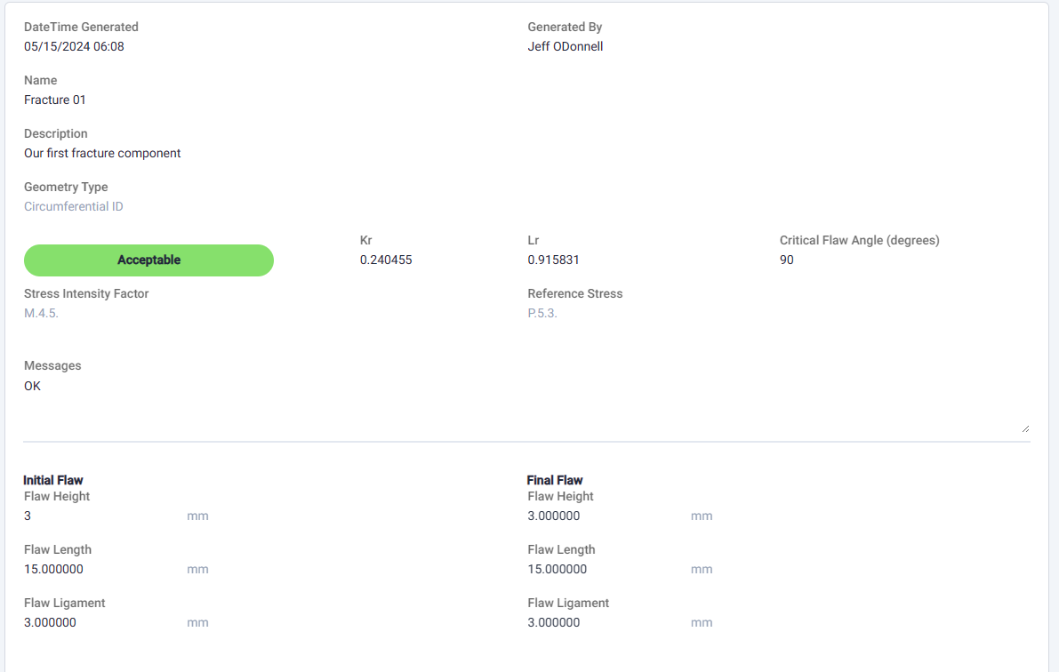


The detailed results page, shown here, is like the one we looked at earlier for surface flaws, but there are a few differences. The solutions chosen for Stress Intensity Factor are those associated with appropriate embedded flaws. The Stress Intensity Factor Details table now calculates Kr values and intermediate values on every line, representing 46 angles between 0 and 90 degrees, as shown below.

Running the Solver and Viewing the Results
This will serve as an introduction to the Solver, and another article will provide a more detailed description. The solver identifies the line on the flaw height vs flaw length chart separating flaws that are acceptable from flaws that are not acceptable – flaws along this line are the Critical Flaws.
Return to the Component, scroll to the bottom, and click the Run Solver button.
This brings up the Solver Setting form. Under Solver Resolution, select High Resolution, and click the Run Solver button. This will assess a surface flaw. To assess an embedded flaw, select Embedded Flaws and input the desired flaw ligament.

The job will be processed, and the results will be sent to the Results page. Navigate to the results page and identify the most recent item. Notice, the icon for Solver Results is different that the icon for regular results.
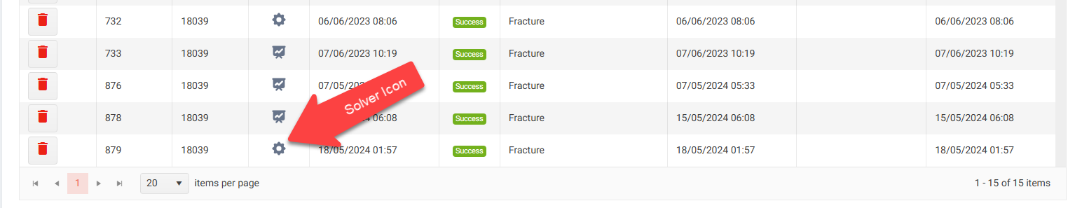
Click on the results line to open the Solver Results. The Solver Results chart illustrates the more than 3000 points assessed to identify the line associated with the critical flaws. In High Resolution, there are 100 points along the critical flaw size line having flaw length to flaw height ratios between 2 to 100. The accuracy of the line is 0.001mm. In Normal Resolution, there are 25 points along the line, and the accuracy of the line is 0.01mm.

The chart is interactive. Hovering the pointer over a point will display the following details: flaw length, flaw height, flaw ligament, flaw angle, whether acceptable, and whether critical.
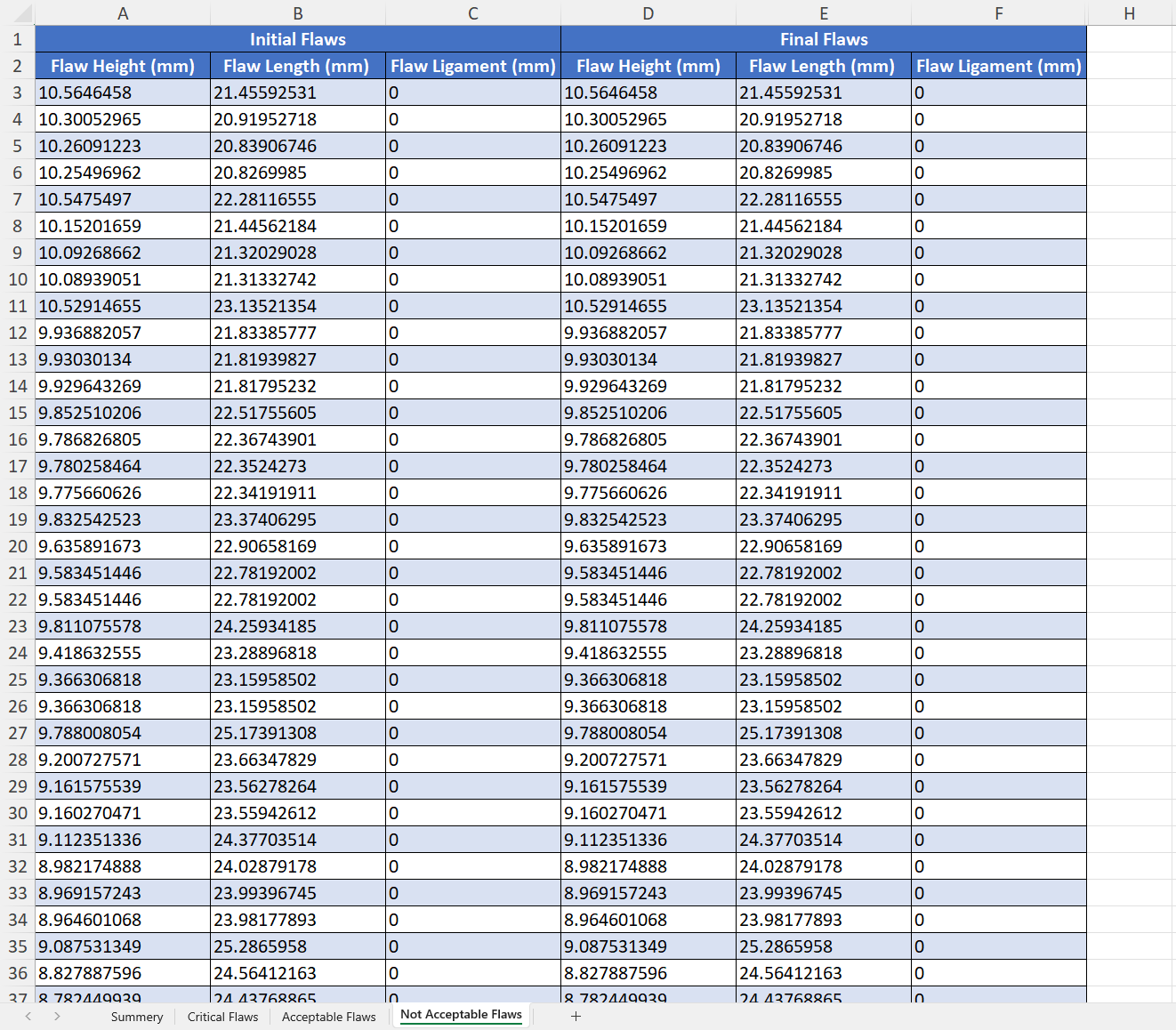
When the user clicks Export As Excel, Material ECA formats the Solver Results as an Excel file and save it to your Downloads folder (depending on the local settings). The Solver Results Excel file has 4 worksheets: Summary, Critical Flaws, Acceptable Flaws, and Not Acceptable Flaws.
The Summary worksheet summarizes the details about the Component and the Solver.

The Critical Flaws page lists the initial and final flaw sizes of those flaws along the Critical Flaw line. As mentioned earlier, the final flaws are the same as the initial flaws, which is not the case for Fatigue and Tearing components, which have some flaw growth.

The Acceptable Flaws page lists the initial and final flaw sizes of all the flaws that were assessed to be Acceptable.

The Not Acceptable Flaws page lists the initial and final flaw sizes of all the flaws that were assessed to be Not Acceptable.
Running a Batch of Flaws and Viewing the Results
The Run Batch allows for the assessment of multiple flaws in a single run in parallel. For this example, we will assess the 100 Critical Flaws calculated from the previous section.
Return to the Component, scroll to the bottom, and click the Run Batch button.

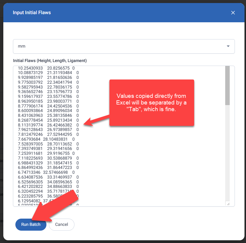
This brings up the Input Initial Flaws form.
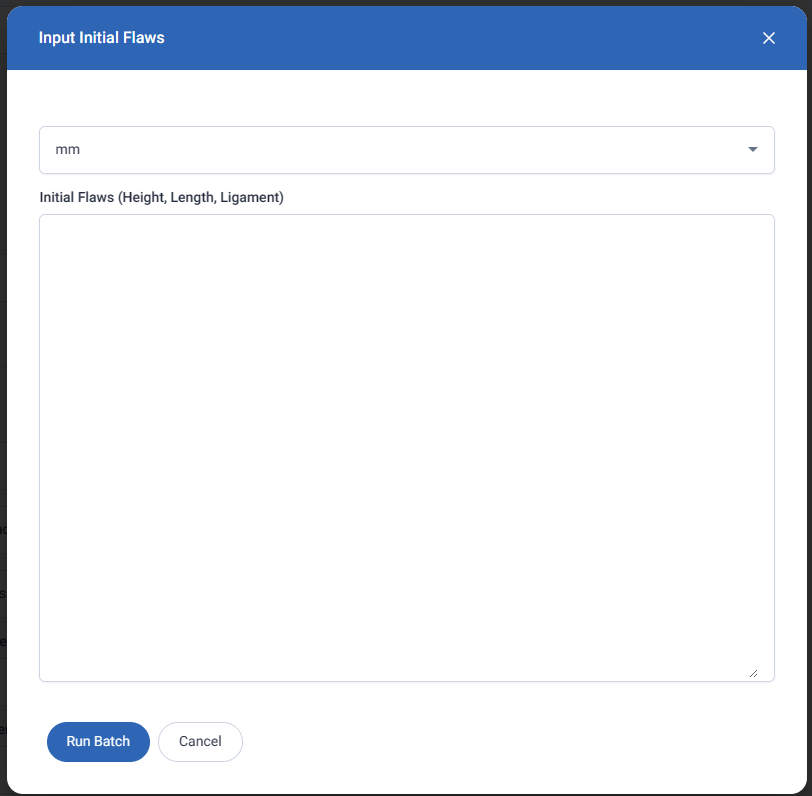
Return to the Solver Results Excel file, on the Critical Flaws page, copy values in the three columns for Flaw Height, Flaw Length, and Flaw Ligament associated with the Initial Flaws (do not copy the column headers), and paste the values into the Initial Flaws text box on the Input Initial Flaws form.

Values paisted directly from Excel will be separated by a “Tab”, which is fine. Material ECA recognizes Tabs, spaces, and commas. The values in each row must be for Flaw Height, Flaw Length, and Flaw Ligament, in that order. Also, confirm the units (mm or inch) is set appropriately.
Click the Run Batch button and navigate to the Results page. The job will be processed, and the results will be sent to the Results page. Navigate to the results page and identify the most recent item.
Click anywhere on the results line to open the Batch Results.
The Batch Results screen has three sections: the summary, the Failure Assessment Diagram, and the Batch Item Results table.
The Failure Assessment Diagram provides the assessment points for all assessed points. Since these are critical flaws, each lies on the Failure Assessment Line. Again, this chart is interactive. Details for each point are provided when hovering the mouse pointer over the point of interest.
The Batch Item Results table provides more details about each assessed point in tabular form. These results can be exported as an Excel File or as JSON for further processing.


Creating a Second Fracture Component by Duplicating and Editing the First
This procedure is a rapid way to create multiple Components for sensitivity assessments, etc.
Navigate to the Components page, identify the Component you want to duplicate, and click the ellipsis (three dots) as shown here.

This will display additional options: Duplicate Component and Delete Component. Select Duplicate Component.

The Duplicate Component form will appear. Rename the component, modify the description, and click the Save button.
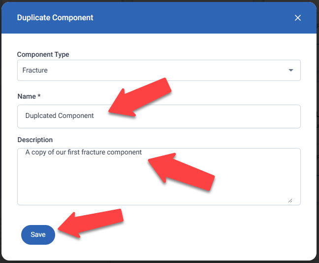
You will be returned to the Components page, and the newly created Component can be found.
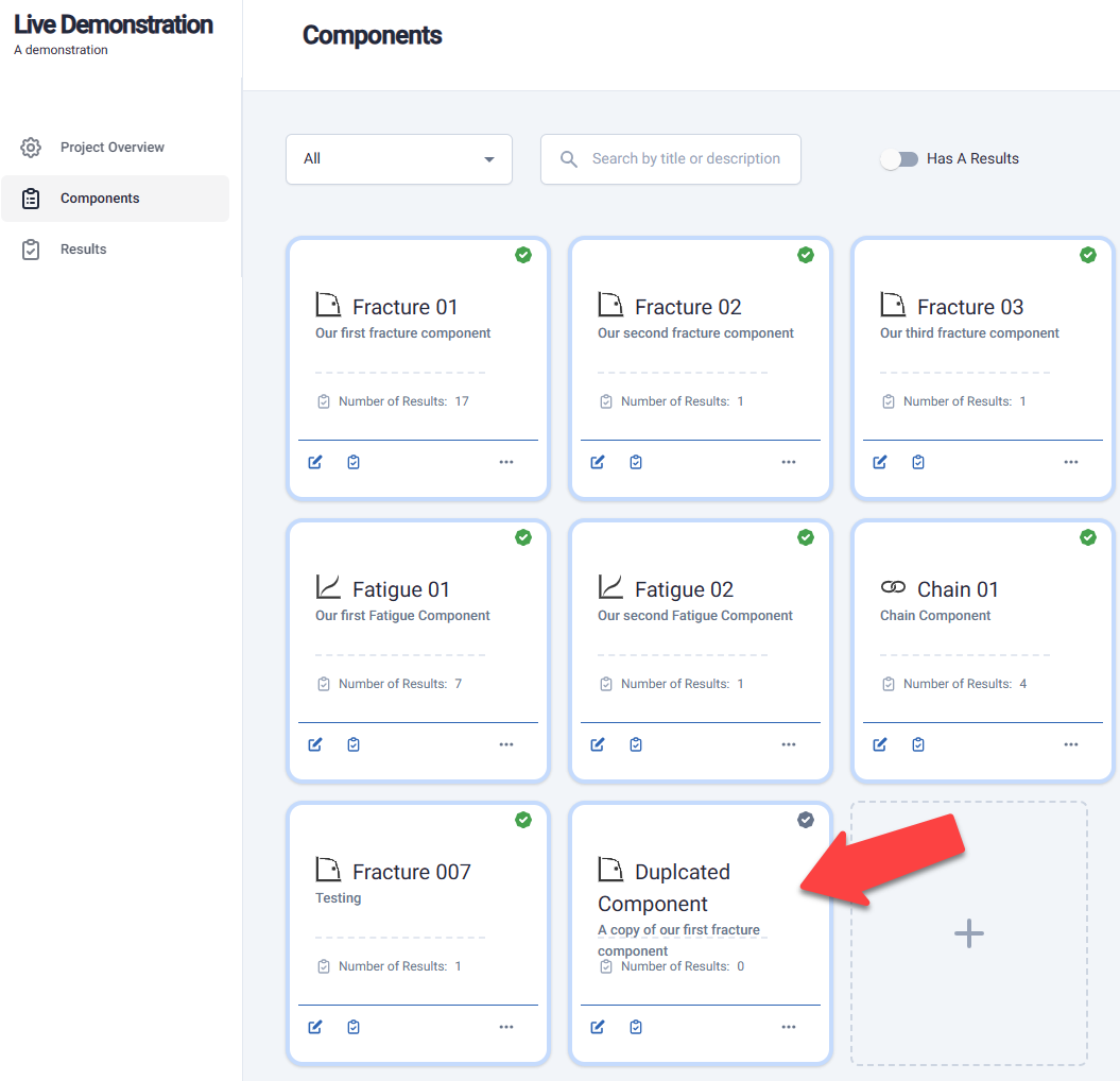
Click on the Duplicated Component tile to open it, modify it as desired, and run it.
Next Article is The Material ECA Solver | Fast and Accurate Assessment of Critical Flaws
The article was last updated on 29 May 2024