The BS 7910 Fatigue Component | Deep Dive

In This Article
The BS 7910 Fatigue component automates the methods described in BS 7910:2019 for fatigue crack growth. This article provides a detailed description about how to use the component, how the component works, its options, and settings. It also introduces the Max Flaw Size component, which can be used with a Fatigue component to provide custom limits to flaw growth. It is assumed the reader is familiar with the Material ECA BS 7910 Fracture component; if not, please read the article for that component before reading this one. The user is expected to be familiar with BS 7910 and should reference their own copy of the document, as appropriate. The topics are covered in this article include the following:
- Overview
- Implementation of the BS 7910 Solutions
- Implementing the Fatigue Crack Growth Solutions
- Creating a New Fatigue Component
- Geometry Input and Options
- Loading and Histogram Input and Options
- Fatigue Crack Growth Law Input and Options
- Fatigue Settings
- Running a Fatigue Component and Viewing the Results
- The Fatigue Report
- Exporting Results to MS Excel
- Tuning the Fatigue Component by Setting the Total Increments
- The Max Flaw Size Component
- Using a Max Flaw Size Component in a Fatigue Component
- Running an Initial Embedded Flaw Using Recharacterization
- Viewing the Results as JSON
- Running the Solver and Viewing the Results
- Creating a Second Fatigue Component by Duplicating and Editing Another
Overview
The BS 7910 Fatigue component assesses the growth and acceptability of an initial crack-like flaw consistent with the methods described in BS 7910:2019 Clause 8 based on stress intensity solutions described in Annex M. In general, each Fatigue component has a cyclic stress histogram and the number of times the histogram is to be applied. For each line in the histogram, cyclic stress intensity values at the surface and deepest points of semi-elliptical, surface flaws, or the extreme points of the major and minor axis of elliptical, embedded flaws are calculated, and the appropriate fatigue crack growth law is used to return incremental growth for the points. Flaw growth is updated continually and proceeds until either the histogram has been applied the desired number of times or the flaw size reaches the maximum size allowed. The maximum flaw size can be set by using a Max Flaw Size Component, which includes a line on a flaw height vs flaw length chart. If the flaw grows beyond that line, the flaw growth calculations end, and the run is Not Acceptable. If no Max Flaw Size Component is used, the maximum flaw size is associated with the validity limits for the solutions associated with the Geometry Type.
Each Fatigue Component can be run using either an initial surface or embedded flaw (depending on the Geometry Type). Analogous to the Fracture component, different fatigue crack growth laws can be input for surface and embedded flaws. In addition, for initial surface flaws multiple fatigue crack growth laws can be input based on distance from the surface, to address, for example, fatigue crack growth through a layer of cladding into the substrate material. The Fatigue component has a helper to rapidly input fatigue crack growth laws recommended by BS 7910:2019. Finally, Fatigue Components have an option to allow embedded flaws to recharacterize as surface flaws when the embedded flaw grows to the surface, as described in BS 7910:2019, Annex E.
Implementation of the BS 7910 Solutions
BS 7910:2019 provides several methods for calculating the cyclic stress intensity factor (DK) depending on the Geometry Type selected. The Geometry Type property is more thoroughly described in the article for Material ECA Components. The following table lists the Geometry Types available, and the BS 7910 solutions used by Material ECA for each.
| Geometry Type | Flaw Type | Cyclic Stress Intensity Factor Solution |
| Plate | Surface | M.4.1 |
| Embedded | M.4.5 | |
| Plate Corner | Surface | M.5.1 |
| Circumferential OD | Surface | M.6 or M.7.3.4 |
| Embedded | M.4.5 | |
| Circumferential ID | Surface | M.6 or M.7.3.2 |
| Embedded | M.4.5 | |
| Axial OD | Surface | M.6 or M.7.2.4 |
| Embedded | M.4.5 | |
| Axial ID | Surface | M.6 or M.7.2.2 |
| Embedded | M.4.5 | |
| Round Straight | Surface Straight | M.10.1 |
Implementing the Fatigue Crack Growth Solutions
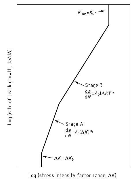
BS 7910:2019 Clause 8 recommends 2 stage fatigue crack growth laws for steels. The following figure from BS 7910:2019 shows the two stages: A and B. When the cyclic stress intensity factor (DK) is larger than a transition value, Stage B fatigue crack growth laws apply, otherwise Stage A fatigue crack growth laws apply. When DK is less than a threshold value, there is no fatigue crack growth. BS 7910:2019 allows for simplified (one stage) and custom fatigue crack growth laws having more stages. Material ECA supports all that flexibility.
Creating a New Fatigue Component
A Fatigue component is created the same way a Fracture component is created. From the Components page, click the tile with the plus (+) sign. In the Add New Component form, select “Fatigue”, “BS 7910:2019”, add a name and description, and click Save, as shown in here.

The newly created Fatigue component is available on the Components page. Click it to open it.
Geometry Input and Options
Geometry input and options are like those for the Fracture component, as shown in the following figure. Let’s provide input like what was done for the Fracture component article.

Loading and Histogram Input and Options
BS 7910:2019 Clause 8 provides guidance for processing a histogram for fatigue crack growth assessments. As shown on the following illustration, the Histogram Table input should have three numerical values on each row in the following order: 1) number of cycles, 2) DPm, and 3) DPb. The numerical values on each row may be separated by any combination of space, comma, or tab. The histogram shown here was copied and pasted directly from an MS Excel table, where the default separator is a tab. This example histogram has 100 rows, and I’ve included it at the end of this article for reference. The Histogram Table input field has a scroll bar on the right side, and its size can be adjusted using the handle on the bottom right.
The “Number of times to apply the histogram” should be a number reflecting the number of times the histogram should be applied. For example, if the histogram represents a year, which is typical for many offshore systems, and the desired lifetime is 20 years, then “20” should be input. If a factor on life of 5 is used, then the input should be “100”, as in this example.

The “Total number of increments” input allows the user to tune the fatigue crack growth calculation. If this number is too low, the fatigue crack growth calculation may not be as accurate. It takes a numerical value larger than the value input for “Number of times to apply the histogram”. In this example, 1000 is input, so the calculation goes through the histogram 1000 times, instead of 100 times. However, each time it goes through the histogram, it proceeds row to row, top to bottom, but for the incremental fatigue crack growth calculations, it uses a value for Ncycles that’s one tenth (0.1) the value for Ncycle input on each row (100/1000 = 0.1), keeping the total number of cycles the same. Tuning the calculation is discussed later in this article.
Fatigue Crack Growth Law Input and Options
Fatigue crack growth laws must be input for both surface and embedded flaws, as shown here:

The Start Height value and unit inputs are only needed for assessments involving non-homogeneous fatigue crack growth and can be ignored otherwise.
The default input is the BS 7910 recommended fatigue crack growth law for steel in-air, mean plus two standard deviations, and R-ratio = 0.5. In the row for Stage A, the Start DK value establishes the threshold cyclic stress intensity value. In the row for Stage B, the Start DK value establishes the cyclic stress intensity value above which Stage B fatigue crack growth laws are used. Click the plus “+” button to add Stage C. Click the minus “-” button to remove Stage B.
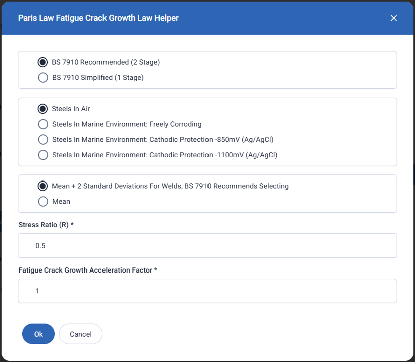
Clicking on the Helper button brings up a form allowing the user to quickly choose and apply one of the fatigue crack growth laws from BS 7910:2019.
Fatigue Settings
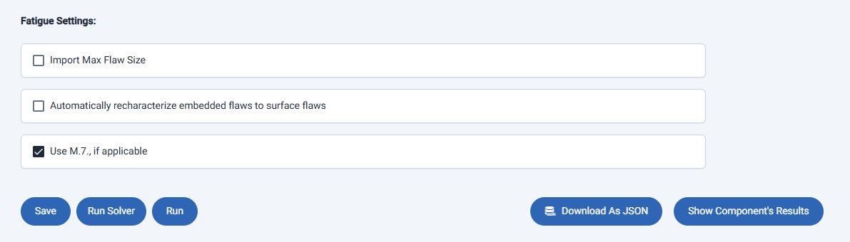
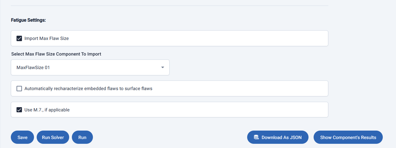
The option to Import Max Flaw Size allows the user to set a custom maximum flaw size by importing a Max Flaw Size component. The Max Flaw Size Component is discussed later in the article. Because the option is not selected, the fatigue crack growth calculations proceed until either the desired number of histograms are processed, or the flaw grows larger than permitted for the Geometry Type.
The option to Automatically recharacterize embedded flaws to surface flaws, allows embedded flaws to be recharacterized as surface flaws when the embedded flaw ligament becomes too small. Recharacterization is accomplished using the method described in BS 7910:2019 Annex E. Embedded flaw recharacterization is discussed later in the article.
The option to Use M.7, if applicable is for initial surface circumferential and axial, ID and OD Geometry Types, where BS 7910: Annex M provides two solutions: M.6 and M.7. The solutions in M.7 are more limiting in scope. Choosing this option instructs Material ECA to use the M.7 option if it’s applicable, otherwise it uses the M.6 solution. If the option is not selected, the M.6 solution is used.
The buttons at the bottom work the same way they work for the BS 7910 Fracture Component.
Running a Fatigue Component and Viewing the Results
Click the Run button, and the Input Initial Flaw form appears. Input the desired initial flaw, as shown, and click the Run button.

Navigate to the Results page for the component and click anywhere on the row associated with the current result to view it. The top of the Results view shows the run was completed successfully and the final flaw was acceptable. The initial and final flaw sizes are provided next.

The flaw growth chart is dynamic; the user can hover the cursor over the curve to see the coordinates for every point. Below the chart are additional details, like those provided in results for Fracture components; however, start and end values are provided for some to indicate if they change during the calculation. Next are the buttons, which are like those for the results for the Fracture component.

The Fatigue Report
Clicking the View Report button generates a document suitable for documenting the run. It provides details of the input and summarizes the results. It can be exported as a PDF file.
Exporting Results to MS Excel
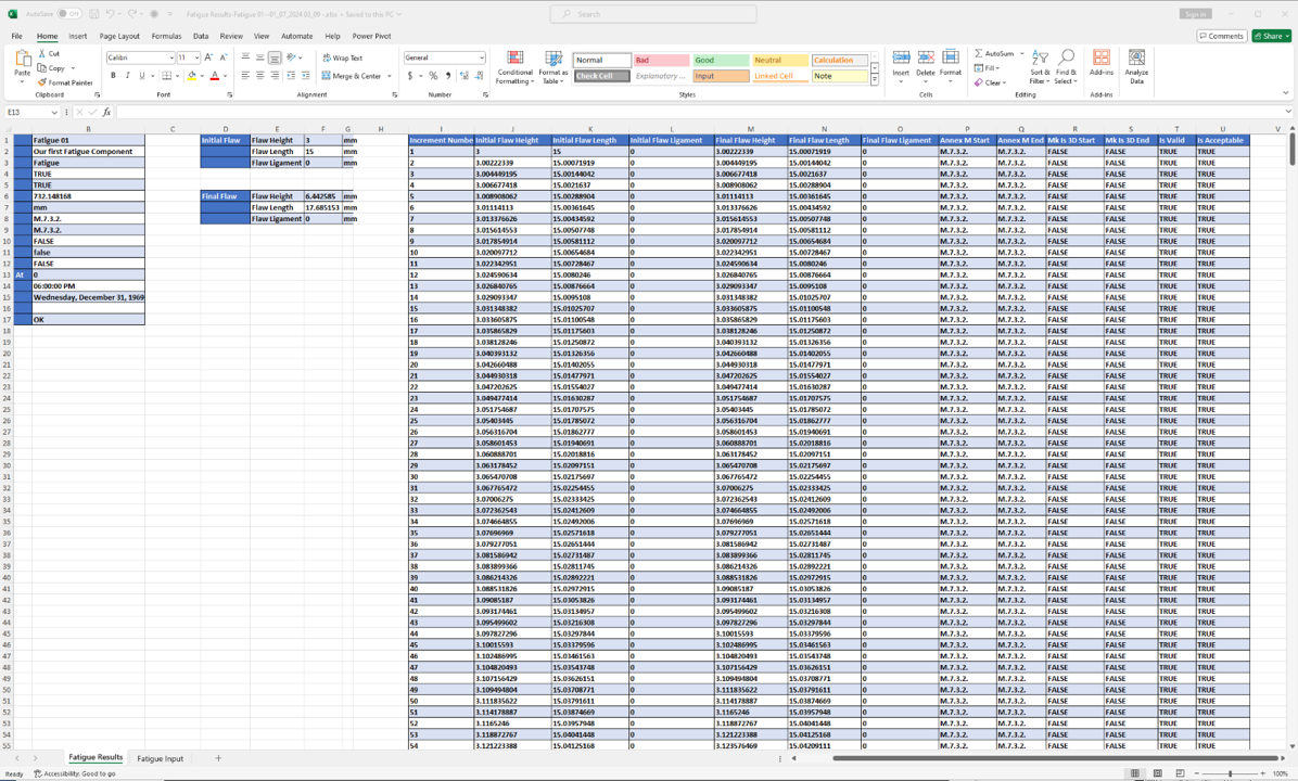
Clicking the Export As Excel button formats the results into an MS Excel file and saves it to the Downloads folder on the local computer, based on the settings. The Workbook has two worksheets: Fatigue Results, and Fatigue Input. The Fatigue Results Worksheet is shown here. It contains a table providing details for each increment, which is 1000 rows in this example.
Tuning the Fatigue Components by Setting the Total Increments
The final flaw size returned has some variation depending on the input total number of increments and the order of the rows in a histogram. There are several ways to tune the fatigue component. A typical approach is described here.
First, sort the rows of the histogram such that the DPm values are ascending (increasing from minimum to maximum). I do this in an Excel worksheet, copy the histogram, and paste it into the Component. Then set the Total number of increments to equal the Number of times to apply the histogram. This is the minimum value. Run the Solver for a surface flaw using high resolution and look at the results. Choose a critical flaw where the ratio (flaw length to flaw height) is between 5 and 10 and record the flaw length (2c). Repeat this for incrementally larger values of Total Number of Increments, such as 400n 700, 1000, 1500, and 2000.
Next, sort the rows of the histogram such that the DPm values are descending (decreasing from maximum to maximum), and repeat the steps described above. List the results in a table and chart it as shown below.

As expected, the difference between the flaw length values for ascending and descending decreases as the Total Number of Increments increases. Also, the histogram with the ascending DPm values predicted a slightly larger final flaw size than the other histogram did. For our example a value of 1000 (which is 10x the Number of Times to Apply the Histogram) was used for the Total Number of Increments; it has a difference of about 0.0035mm. Note: the Solver’s accuracy using High Resolution is 0.001mm. We also used an ascending histogram, so it should be expected to be appropriately conservative.
While this assessment found the Total Number of Increments 10x the Number of Times to Apply the Histogram was reasonable, some histograms require significantly more to get the same levels of accuracy.
The Max Flaw Size Component
The Max Flaw Size component is a lightweight, utility Material ECA Component allowing Users to quickly and easily provide custom limits on flaw size in terms of flaw height and flaw length. It can be used in Fatigue components to limit fatigue crack growth, as discussed in this article, or it can be used in Chain and Group components, as desired. Since the Max Flaw Size component is independent of other components, it can be used in any number of Fatigue, Chain, and Group components. However, please understand that making changes to a Max Flaw Size component impacts every component that uses it. A common way to use Max Flaw Size component is based on the Solver results associated with Fracture components or Group components that use numerous Fracture components, which represent the critical end-of-life flaw sizes.
Max Flaw Size components are created the same way other Components are created. From the Components page and click the tile with the plus (+) symbol. In the Add New Component form, for Component Type, scroll down and select Max Flaw Size, enter a name and description, and click the Save button. Return to the Component page and open the newly created Max Flaw Size component. Set the Geometry Type to Circumferential ID, to match the Geometry Type of the Fatigue component, see below.

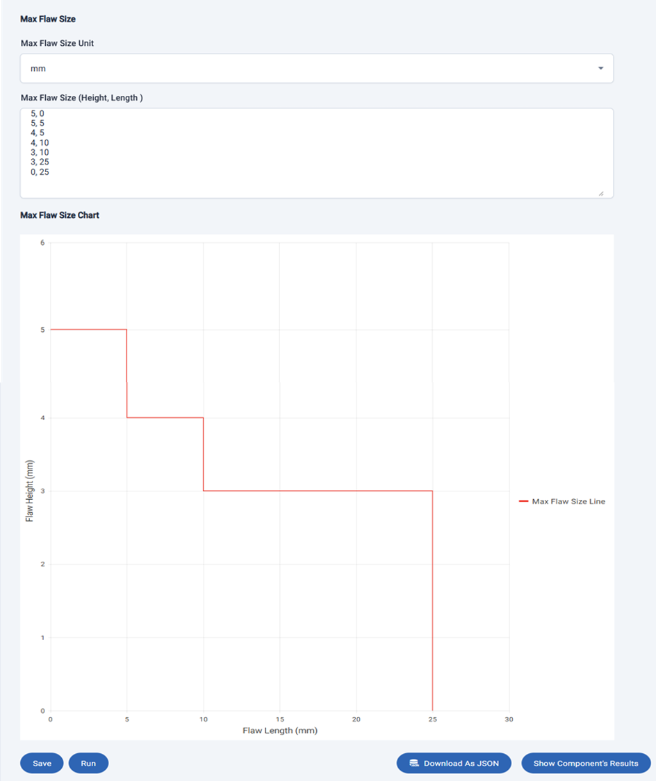
Input the points as follows and shown below to set the Max Flaw Size line, and set the unit to mm.
- 5, 0
- 5, 5
- 4, 5
- 4, 10
- 3, 10
- 3, 25
- 0, 25
Each row represents a point and has two values: the first value is the flaw height, and the second value is the flaw length. Like the Histogram input, the two values must be separated by either a comma, space, or tab.
The associated line appears in the Max Flaw Size Chart. The points must have the following properties:
- The first point must have a flaw length of 0
- The final point must have a flaw height of 0
- No line segment may have a positive slope
Click the Save button and return to the Components page.
Using the Max Flaw Size Component in the Fatigue Component
Return to the Fatigue component we have been working with, scroll to the bottom, and under Fatigue Settings, select the Import Max Flaw Size check box. A dropdown input field appears, click on it and select the newly created Max Flaw Size component. Click the Save button.
Click the Run button, input an initial flaw height of 2.5mm, initial flaw length of 15mm, initial flaw ligament of 0 (for a surface flaw), and click the Run button. Navigate to the Result page and open the associated Result, see below. The initial flaw is Not Acceptable, the run stopped after increment 257 of 1000, and the final flaw had a height just less than 3mm, consistent with the input Max Flaw Size.
Max Flaw Size components work the same way with embedded flaws. Regardless of the ligament, when the embedded flaw size in terms of height (2a) and length (2c) reaches the Max Flaw Size limit the Fatigue run stops, and the initial flaw is Not Acceptable.

Running an Initial Embedded Flaw Using Recharacterization
Return to our Fatigue component, scroll to the bottom, deselect the Max Flaw Size option, select the Automatically recharacterize embedded flaws option, and click the Run button. Input an initial embedded flaw having a Flaw Height of 6mm, Flaw Length of 25mm, a Flaw Ligament of 3mm, and click the Run button. The Results are shown here:

The initial embedded flaw was Acceptable and it recharacterized as a surface flaw at increment 572 of 1000. Click the Export As Excel button, and open the Excel file to view the details of the recharacterization, shown here:

Viewing the Results as JSON
Return to the Results, scroll to the bottom, and click the Export As JSON button. This creates a text file with the results data formatted as JSON and saves it to your Downloads folder on your local computer.
JSON is an open-standard, lightweight data format for storing and transporting data commonly used to transport data between apps on local devices (i.e., phones, tablets, computers) and servers. It is quickly and easily read by most modern programming languages and by humans using a text editor. The official JSON site is JSON.org, and there are countless websites describing JSON and how it can be used. A powerful feature of Material ECA is that Components can be programmatically generated and imported to Material ECA as JSON data, and Material ECA results can be exported as JSON so they can be programmatically processed by other digital systems and platforms.
To view JSON data, I usually use the Edge browser with the JSON Formatter extension, shown here:

Expanding the Input item reveals all input data, and expanding the IncrementDetails reveals the details for all 1000 increments. Coded enumerations are used for some properties, including ComponentType, MmMbType (which references the applicable paragraph in Annex M), and all Units. These are described in detail in the JSON article.
Running the Solver and Viewing the Results
Running the Solver on a Fatigue component is no different than running the Solver on a Fracture component, and the Results are formatted the same way. For more information, see the articles on the Fracture Component and the Solver.
Creating a Second Fatigue Component by Duplicating and Editing the First
A Fatigue component can be quickly duplicated the same way a Fracture component can be duplicated. From the Components page, on the tile for the Component to duplicate, click on the ellipsis (3 dots) in the bottom right corner of the tile, and then click on the Duplicate Component item on the menu that appears.
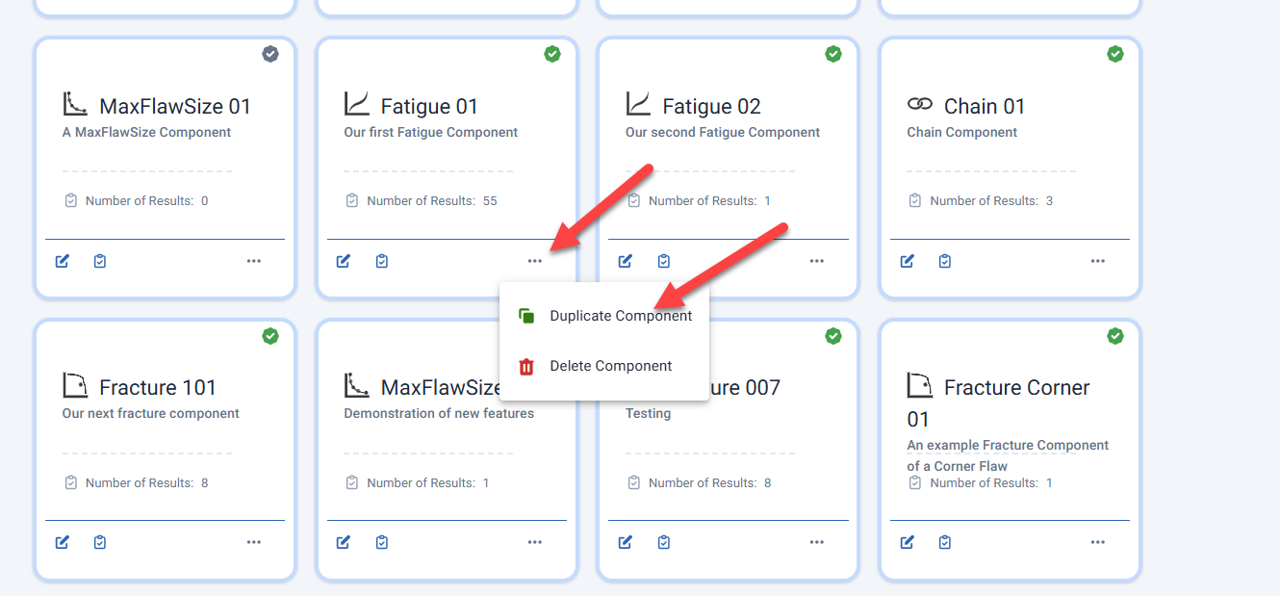
A new Fatigue Component appears, open it, rename it, give it a meaningful description, and edit it as desired.
Example Histogram as comma separated values
Ncycles, DPm (MPa), DPb (MPa)
5308338.25, 0.34, 0
474595.5, 1.03, 0
171574.25, 1.72, 0
107469.25, 2.41, 0
72220, 3.1, 0
55310.5, 3.79, 0
40956.5, 4.48, 0
34115.75, 5.17, 0
26291.75, 5.86, 0
20865.75, 6.55, 0
18711.75, 7.24, 0
16648.5, 7.93, 0
14447.75, 8.62, 0
12573.25, 9.31, 0
11015.75, 10, 0
8578.5, 10.69, 0
10076, 11.38, 0
7560, 12.07, 0
7319.5, 12.76, 0
6687.5, 13.44, 0
4804.5, 14.13, 0
4295, 14.82, 0
4603.25, 15.51, 0
3792.5, 16.2, 0
3359.5, 16.89, 0
3320.25, 17.58, 0
2816.5, 18.27, 0
2966.75, 18.96, 0
2794.25, 19.65, 0
2140, 20.34, 0
1779.5, 21.03, 0
1725, 21.72, 0
1603, 22.41, 0
1292, 23.1, 0
1256, 23.79, 0
1285.25, 24.48, 0
1305.25, 25.17, 0
1004.25, 25.86, 0
1201.25, 26.54, 0
946.75, 27.23, 0
712, 27.92, 0
1491.25, 28.61, 0
949.25, 29.3, 0
648.75, 29.99, 0
639.75, 30.68, 0
1088, 31.37, 0
493.25, 32.06, 0
482.5, 32.75, 0
408.75, 33.44, 0
579.5, 34.13, 0
387, 34.82, 0
203.25, 35.51, 0
465, 36.2, 0
327.25, 36.89, 0
290.75, 37.58, 0
295.25, 38.27, 0
1009.5, 38.96, 0
310, 39.64, 0
226.75, 40.33, 0
190.5, 41.02, 0
181.25, 41.71, 0
159.25, 42.4, 0
155.5, 43.09, 0
76.5, 43.78, 0
135.5, 44.47, 0
93.5, 45.16, 0
82.5, 45.85, 0
90.25, 46.54, 0
128.75, 47.23, 0
50, 47.92, 0
85.5, 48.61, 0
111.75, 49.3, 0
78.5, 49.99, 0
34.5, 50.68, 0
28.75, 51.37, 0
29.75, 52.06, 0
30.25, 52.74, 0
19.5, 53.43, 0
12.75, 54.12, 0
19.25, 54.81, 0
11.25, 55.5, 0
17.5, 56.19, 0
95, 56.88, 0
242.75, 57.57, 0
10, 58.26, 0
9.25, 58.95, 0
7.25, 59.64, 0
7.75, 60.33, 0
1.75, 61.02, 0
5.5, 61.71, 0
1.25, 62.4, 0
0.25, 63.09, 0
1.75, 63.78, 0
3.25, 64.47, 0
1, 65.16, 0
0.25, 65.84, 0
0.25, 66.53, 0
0.25, 67.22, 0
5.5, 67.91, 0
Next Article: The BS 7910 Tearing Component | Deep Dive
Last Modified: 04 July 2024